gnuplot 語法解說和示範
tags: sysprog2017
解說影片: 輕輕鬆鬆學 gnuplot
在作業中常需繪製圖表以更清楚的說明及展現實驗結果,gnuplot 就是一個好用的工具,以下會說明一些寫 ==gnuplot script== 的相關技巧
gnuplot 指令
gnuplot script 副檔名為 .gp
繪圖︰$ gnuplot [script 檔名] 檢視圖片︰$ eog [圖檔名]
結合進 Makefile 中會更方便! 以 phonebook 中的 Makefile 為例:
plot: output.txt (tab) gnuplot scripts/runtime.gp[color=red]
繪圖時直接下指令
$ make plot就好囉!
gnuplot script
-
設定 還有更多設定可以自由變換組合,下面提供較為常見的設定
#: 註解行reset: 重新設定set term png enhanced font 'Verdana,10': 設定圖片類型set output 'runtime.png': 存檔名稱set logscale {x,y}: 設定 X 或 Y 軸或是兩者為 logscaleset xrange [a:b]: 設定 X 軸範圍從 a 到 b (Y 軸亦可);若是看不到圖形,可用 set autoscale 自動調回set xlabel "XXX", a,b: 設定 X 軸的名稱為 XXX (Y 軸亦同), 從預設向右移動 a,向上移動 bset xlabel "XX" font "Times-Italic,26": 設定X軸的名稱為 XX,以 Times-Italic 字型大小 26set title "GGG": 設定圖形標題為 GGGset xtics a: 設定顯示的 X 軸座標與刻度, 每次增加 a ;在 logscale 時,預設的設定會沒有小刻度set xtics a,b: 設定顯示的 X 軸座標與刻度 起始值 a,每次增加 bset format y "10^ { %L } ":Y 軸的值以 10 的 L 次方顯示set format x "%a.bf": X 軸的值以總長 a 位數,小數點以下 b 位顯示set format x "%a.be": 以科學記號顯示set format x "": 不顯示X軸的座標值set key Q,W Left reverse: 將圖例與曲線標題倒過來放在圖上座標 (Q,W) 處set key spacing D: 設定圖例間的寬度增加 D 倍set key title "XXX": 設定圖例的名稱set label "SSS" at Q,W: 設定 SSS 這三個字出現在座標(Q,W)處set label "XX" textcolor lt 2: 以linetype 2 顯示 XXset grid: 在各主要刻度畫出格子
-
繪製
plot後面就緊接著一連串繪圖指令,gnuplot 會依照程式碼的順序繪圖,因此沒設定好會有覆蓋的情形。
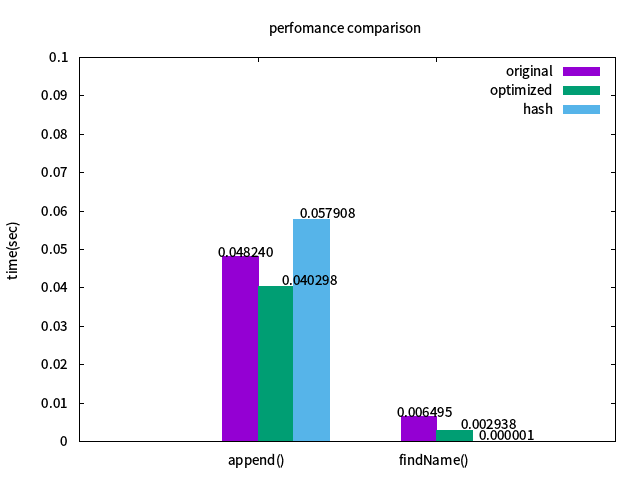
讓我們以 phonebook 作業中的 runtime.gp 為例說明
output.txt:
append() 0.048240 0.040298 0.057908
findName() 0.006495 0.002938 0.000001
runtime.gp:
- 讀取 output.txt 的資料繪圖且 Y 軸的範圍設定為 0~0.100
- 讀第二個 column (等同於 using 1:2) 的資料,而第一個 column 為 X label
- 繪製成 histogram 且 名稱為 original
'': 因使用同一個output.txt檔,所以可以簡寫(易等同於'output.txt')
plot [:][:0.100]'output.txt' using 2:xtic(1) with histogram title 'original', \
'' using 3:xtic(1) with histogram title 'optimized'  , \
'' using 4:xtic(1) with histogram title 'hash'  , \
- 調整資料顯示位置, $0 為 "pseudo-columns"
The sequential order of each point within a data set. The counter starts at 0 and is reset by two sequential blank records. The shorthand form $0 is available.
+or-的值皆為位移量$2 $3..: 就是第二個 columm,第三個 column 以此類推
'' using ($0-0.06):($2+0.001):2 with labels title ' ', \
'' using ($0+0.3):($3+0.0015):3 with labels title ' ', \
'' using ($0+0.4):($4+0.0015):4 with labels title ' '
:::danger gnuplot 繪製同一來源檔案時指令應為不中斷的一大長串,我們可以使用\連接各行排版,提高可讀性 :::
美圖欣賞
- 輸出 runtime.png:
 對應的程式碼
reset
set ylabel 'time(sec)'
set style fill solid
set title 'perfomance comparison'
set term png enhanced font 'Verdana,10'
set output 'runtime.png'

plot [:][:0.100]'output.txt' using 2:xtic(1) with histogram title 'original', \
'' using ($0-0.06):($2+0.001):2 with labels title ' ', \
'' using 3:xtic(1) with histogram title 'optimized'  , \
'' using 4:xtic(1) with histogram title 'hash'  , \
'' using ($0+0.3):($3+0.0015):3 with labels title ' ', \
'' using ($0+0.4):($4+0.0015):4 with labels title ' '
- 善用設定就能得整齊美圖一張
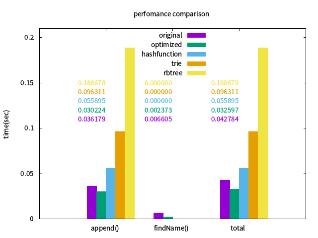
source 對應程式碼:
reset
set ylabel 'time(sec)'
set style fill solid
set key center top
set title 'perfomance comparison'
set term png enhanced font 'Verdana,10'
set output 'runtime.png'

plot [:][:0.210]'output.txt' using 2:xtic(1) with histogram title 'original', \
'' using 3:xtic(1) with histogram title 'optimized'  , \
'' using 4:xtic(1) with histogram title 'hashfunction'  , \
'' using 5:xtic(1) with histogram title 'trie'  , \
'' using 6:xtic(1) with histogram title 'rbtree'  , \
'' using ($0-0.200):(0.110):2 with labels title ' ' textcolor lt 1, \
'' using ($0-0.200):(0.120):3 with labels title ' ' textcolor lt 2, \
'' using ($0-0.200):(0.130):4 with labels title ' ' textcolor lt 3, \
'' using ($0-0.200):(0.140):5 with labels title ' ' textcolor lt 4, \
'' using ($0-0.200):(0.150):6 with labels title ' ' textcolor lt 5
- 分佈圖
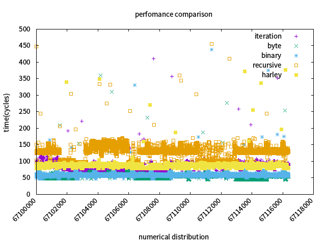
source 對應的程式碼
reset
set xlabel 'numerical distribution'
set ylabel 'time(cycles)'
set title 'perfomance comparison'
set term png enhanced font 'Verdana,10'
set output 'runtime.png'
set format x "%10.0f"
set xtic 2000
set xtics rotate by 45 right

plot [:][:500]'iteration.txt' using 1:2 with points title 'iteration',\
'byte.txt' using 1:2 with points title 'byte',\
'binary.txt' using 1:2 with points title 'binary',\
'recursive.txt' using 1:2 with points title 'recursive',\
'harley.txt' using 1:2 with points title 'harley'
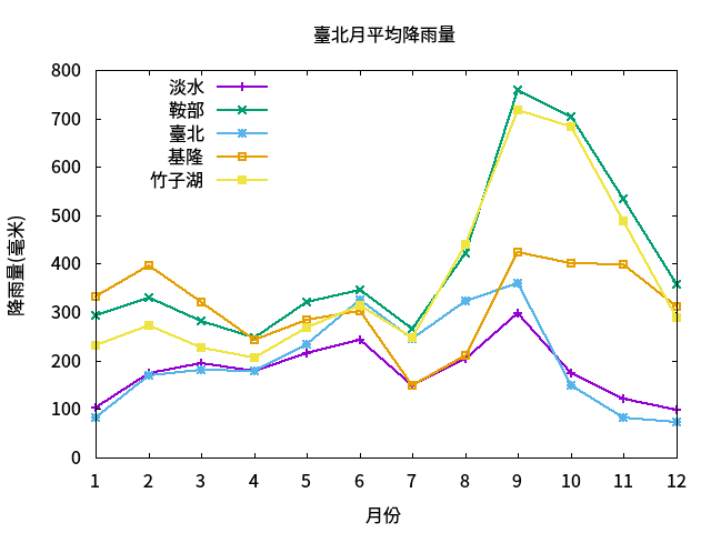
案例探討:臺北年度雨量長條圖
- 資料來源: 臺北地區各氣象站月平均降雨量統計表
#測站  |  淡水  |  鞍部  |  臺北  |  基隆  |  竹子湖  |
#月份
1       103.9   294.3     83.2   331.6    232.6
2       174.8   329.2    170.3   397.0    273.5
3       194.5   281.8    180.4   321.0    227.1
4       179.3   247.9    177.8   242.0    207.2
5       216.1   321.2    234.5   285.1    267.4
6       243.4   345.8    325.9   301.6    314.8
7       149.2   266.1    245.1   148.4    247.7
8       202.9   422.5    322.1   210.1    439.5
9       299.1   758.5    360.5   423.5    717.4
10      173.9   703.5    148.9   400.3    683.9
11      120.7   534.7     83.1   399.6    488.8
12      97.6    357.6     73.3   311.8    289.1
- 準備 gnuplot 的腳本:
set title "臺北月平均降雨量"
set xlabel "月份"
set ylabel "降雨量(毫米)"
set terminal png font " Times_New_Roman,12 "
set output "statistic.png"
set xtics 1 ,1 ,12
set key left

plot \
"data.csv" using 1:2 with linespoints linewidth 2 title "淡水", \
"data.csv" using 1:3 with linespoints linewidth 2 title "鞍部", \
"data.csv" using 1:4 with linespoints linewidth 2 title "臺北", \
"data.csv" using 1:5 with linespoints linewidth 2 title "基隆", \
"data.csv" using 1:6 with linespoints linewidth 2 title "竹子湖" \
- 參考輸出畫面:
參考及引用連結
书籍推荐